The Real EUR of EOG's Bakken Shale Wells
SA author Michael Filloon wrote on the Bakken shale wells of QEP Resources (QEP). He projected an EUR up to 2 million barrels of oil equivalent. I disagree with his calculation. Real production data does not support his conclusion. I pick the first well listed in his article, No. 16637, owned by EOG resources (EOG), for a case study.
Modeling Shale Well Declines
Traditionally natural gas (UNG) producers use the classical Arps formula to model a conventional oil or gas well's production decline.
As I discovered, and as many people pointed out, the classical Arps formula is not suitable for projecting shale well's decline patterns, as shale wells decline much faster than the formula projects in the long term. Specifically the terminal decline of Arps formula approaches zero, and the cumulative production it projects approaches infinity with a b-factor larger than 1.0. That's problematic, as in the long term, shale wells should decline a terminal decline rate above zero.
Let's re-cap about the classical Arps formula and how I modified it:
(click to enlarge)
I am happy to find out that even though most producers insist on using the classical Arps formula, QEP does use the SAME modified Arps formula with a terminal decline term introduced. In that sense they agree with my own modeling method. I congratulate management of QEP for being a little bit more honest than Chesapeake (CHK) and Cabot Oil & Gas (COG).
But even QEP used the same correct modified Arps formula as I do, and admitted a reasonable terminal decline rate, they still pushed for a set of parameters that gave a higher EUR (Estimated Ultimate Recovery) than what is realistically possible.
Modeling Bakken Well No. 16637
I extracted monthly production data from ND DMR web site. I did the calculation on a spreadsheet. Here are the comparisons. Note that both QEP and I used the same formula with four parameters: IP, D, b-factor and terminal decline rate Beta. I just disagree with QEP on what parameters provide the best fit. Here is QEP's model:
(click to enlarge)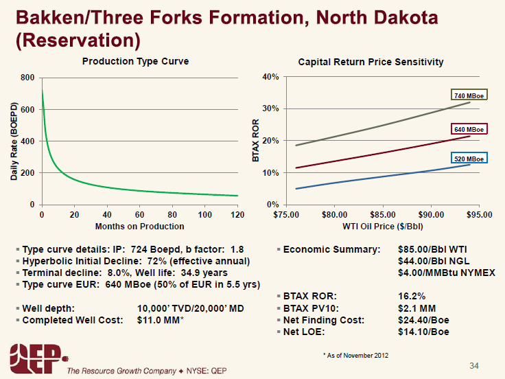
According to the chart, here are QEP's parameters, versus mine:
- QEP adopts IP = 724 BPD, D = 0.0035/day, B = 1.80 and Terminal decline rate Beta = 0.000228/day
- I adopt IP = 1250 BPD, D = 0.020/day, B = 1.80 and Terminal decline rate Beta = 0.000280/day.
As I said, I agree with QEP in the formula used, I disagree with them in the specific fitting parameters. Let's see who fit the data better:
(click to enlarge)
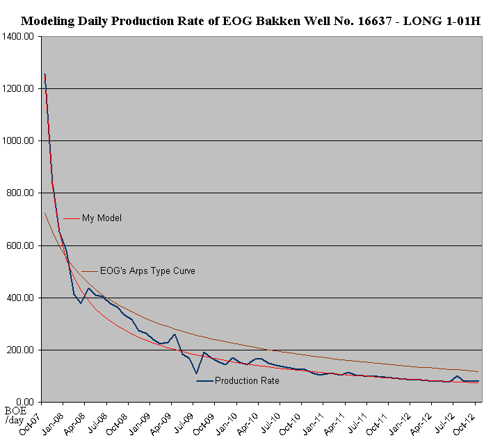
It appears to me that my curve fit the actual production data much better. The QEP curve does not fit the well data very well.
My speculation is that they know that they need a flat curve to obtain a higher EUR value. The more flat the curve is, the higher EUR it will calculate. Thus they probably deliberately pull the IP down to a much lower starting point.
To compensate for a lower starting IP, they adopt a much smaller initial decline rate D, which makes the curve flatter.
Finally, to further flatten the curve, they tried to fit the artificial local peak of production, at April and May of 2008, which resulted from re-fracing operation (re-stimulation). I believe the cur should follow the non-disturbed natural decline trend, instead of following the artificial temporary boost of production, to be realistic.
The chart above shows that my curve following the real production down closely, while the QEP curve deviate on the higher side.
(click to enlarge)

The above chart, plotted in much longer time scale, and using logarithm scale, shows the deviation much better. Once again, my curve tracks the actual production data very closely. But the QEP curve clearly deviates from the real data and projects too high.
As a result, when you integrate the cumulative production over time, QEP's curve would over-estimate while my curve gives the accurate projection. See below:
(click to enlarge)
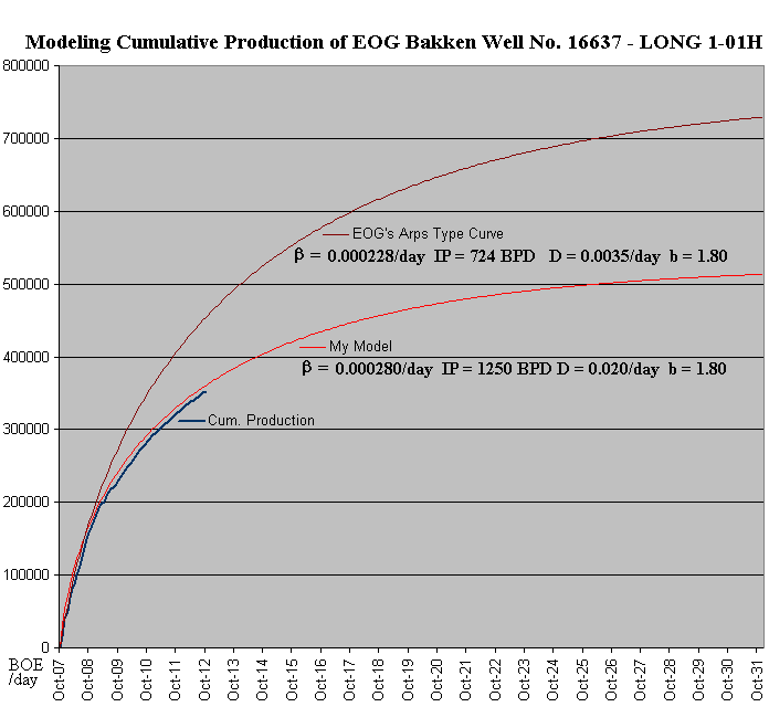
As shown above, my parameters leads to accurate projection of the actual production. The QEP curve clearly deviates on the high side.
I projected that the EIR of well No. 16637 will likely be 500 MBOE. The QEP projection is 750 MBOE. The chart clearly agrees with me.
Calculation and Discussion
As of now, the well 16637 is a bit more than five years old, and has produced an accumulative 355.280 MBOE. Current production rate is 80 BOE/day. Current annual decline rate is -16% to -22%. Using -18% annual decline, and using 10 BPD as cut off, the well will produce another 145 MBOE, bring the total EUR to 500 MBOE.
This well is NOT a typical or average Bakken shale well. If it is, even if the EUR is only at 500 MBOE, producers would make an incredible profit at $100/barrel oil price. Unfortunately that is not the case. The average Bakken shale well has a much lower IP and much lower EUR, even if they are equally cost to drill.
As of October 2012, there are 6349 producing Bakken shale wells. They collectively produced 821.30 MBOE/day. There are 6077 wells which were also producing in September, and 272 new wells which first show up in October. The 6077 wells producing in both months collectively declined from 790.33 MBOE/day to 715.820 MBOE/day from September to October, or -9.5%/month. That is a daily decline rate of /month, or -0.33%/day. At this decline rate, these well's future production will be equivalent to 1/0.33% = 303 days worth of production at current rate of 716 MBOE/day, or 217 million BOE. Divided by well numbers, each well has an average of 35.7 MBOE remaining production. That does not look like a lot of value to me. At $90/barrel, that's a remaining production value of $3.2M each.
Good luck drilling every well as productive as No. 16636, producers!
I repeatedly pointed out that shale oil and gas producers tend to over-exaggerate productivity of their wells, under-estimate the well declines, and under-calculate the fair capital amortization cost, in order to pitch their investment case to banks and investors, so they can keep borrowing more money to keep drilling shale wells.
In reality, even Bakken shale oil wells are hardly profitable at current oil prices and current development costs. My advice to investors is to do your own due diligence research and scrutinize the data. Avoid the hyped shale oil and gas sector. The sector you should get into, is the US coal mining sector. The meme that natural gas is replacing coal, is completely wrong. Natural gas will always be an important part of America's energy supply. But at fair cost, shale gas can not compete with the cheap king coal.
The investment case in coal is made better as nearly 99% of investors made the wrong bet, as there is 75 times more market capital invested in the NG sector than in the US coal sector, while both sectors contribute about equal energy to the US economy.
Imagine what happens when the looming debt crisis in the NG sector unfold, and shale gas production collapses, sending prices of both NG and coal much higher, and 75 more market capital in the NG sector now moves to coal sector instead. This is not an opportunity you get to see every year. Now is the best time to get into coal. I recommend these names: JRCC, ANR, ACI, BTU.

7 comments:
your thesis is valid and your conclusions might well be correct, but your ammunition and starting point could be refined:
you use a source that claims 01 was frequently disallowed. since we agree b=0 is exponential, a source saying 0<b<1 is also exponential ought to be viewed with a bit more skepticism.
one source of a common terminology that also confirms 0<b<1 is hyperbolic would be SPEE REP#06, which we non-members can also use for consistency
https://secure.spee.org/sites/default/files/wp-files/pdf/ReferencesResources/REP06-DeclineCurves.pdf
there may indeed be some in industry, or some blogging authors, who claim it valid to use hyperbolic-only declines that are hyperbolic-to-infinity or even just hyperbolic-to-abandonment. i haven't seen one, but one or more may exist.
unfortunately many use hyperbolic to mean hyperbolic-until-a-terminal-decline-is-reached-and-after-that-something-else.
your approach is an improvement on hyperbolic-to-infinity if anyone is actually using the latter.
you make a strong case your fit is better. you don't claim best, again restraint is good.
it is nice to see your type curve comparison on a cumulative production plot. keep up the good work.
a hyper-skeptic
meant to say
"you use a source that claims 01 was frequently disallowed. since it is agreed b=0 is exponential, a source saying 0<b<1 is also exponential ought to be viewed with a bit more skepticism."
Excellent post
Excellent work, JJ. Did you go into all monthly reports namely, 12* No.of Years each to get just W#16637? or is there some well specific search option? Any CSV downloads? -- Thanks, Moshe
From my perspective as an industry evaluation engineer I think you are oversimplifying it a little bit. Obviously we know you can't use a B factor over 1 for the life of the well, and really hyperbolic doesn't work well for the first few months of production either.
We either use two part curves - that is we model the beginning of the well as hyperbolic and then use an exponential decline after a few years for the tail production.
The beginning few months are so dynamic it is often hard to fit with the rest of the curve. If you are a private operator or bank evaluating then you have the option of just ignoring it until production is more mature. Obviously a public company doesn't have that option so they make a stab at it. The result is that type curves are not as accurate as we would like and revisions do happen from time to time.
there may indeed be some in industry, or some blogging authors, who claim it valid to use hyperbolic-only declines that are hyperbolic-to-infinity or even just hyperbolic-to-abandonment. i haven't seen one, but one or more may exist.
DOOGEE X3 Review
Huawei Enjoy 5S Review
Mpie F5 Specs
Bandar Poker
Qiu Poker
Judi Poker
Ceme Poker
IDN Poker
Poker Online Terbaik
Situs Poker Indonesia
Daftar Poker Online
99 Poker Indonesia
Post a Comment